MachineLayout: Survey and 2D/3D Layout Plotting

This document explains the concepts behind the Ocelot survey and layout tools and how they are intended to be used.

It covers:

1. Beamline geometry surveys using MagneticLattice
2. The meaning of survey output data
3. Why and when to use the higher-level MachineLayout
4. 2D and 3D visualization concepts
5. Interference (collision) checks
6. Practical usage tips

The focus here is on concepts and data structures, not on code details.

---

Overview

In Ocelot, the geometric layout of a beamline or facility is described using a survey. A survey computes the global positions and orientations of beamline elements starting from a given reference point.

Key idea:
The survey determines where the beamline is in the global laboratory frame and how it is oriented at each point.

---

Requirements

• Core survey and layout functionality requires only Ocelot and its numerical dependencies.
• 2D plotting relies on standard plotting libraries.
• 3D plotting (optional) requires Plotly.

If Plotly is not installed, all survey functionality and 2D visualization remain available.

Note:
Plotly is used only for interactive 3D visualization and is intentionally kept outside ocelot.cpbd.

from ocelot import *

# New survey class / plotting
from ocelot.cpbd.layout import MachineLayout
from ocelot.gui.layout_2d import plot_layout_2d
from ocelot.gui.layout_3d import plot_layout_3d

initializing ocelot...

MagneticLattice.survey()

Before introducing the higher-level MachineLayout, it is important to understand the low-level geometric survey provided by MagneticLattice.

For a complete description of the survey algorithm, returned data structures, and conventions, see the MagneticLattice.survey() method documentation.

Here we only consider a simple example showing how to call survey() and how to interpret and visualize the resulting survey data.

---

Simple usage of survey()

For a single beamline, MagneticLattice.survey() is sufficient to:

• inspect global positions and orientations
• verify bending and tilt behavior
• produce simple 2D plots (e.g. top or side views)
• debug element geometry

At this level, the user works directly with the lists of survey dictionaries returned by the method.

import matplotlib.pyplot as plt
lat = MagneticLattice([
    Drift(l=5, eid="d1"),
    Quadrupole(l=0.5, eid="q1"),
    SBend(l=2.0, angle=0.3, eid="b1"),
    Drift(l=4, eid="d2"),
])

mid, end = lat.survey()

print("Number of records:", len(end))
print("Keys in one record:")
print(end[0].keys())

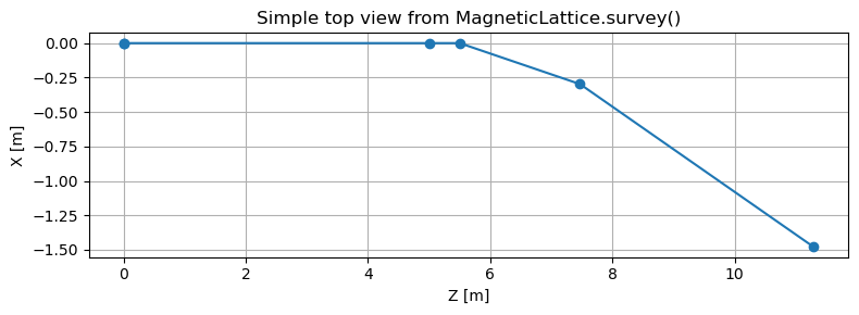
# simple matplotlib plotting

# Extract centerline points
X = [p["r_start"][0] for p in end]
Z = [p["r_start"][2] for p in end]

# add final exit point
X.append(end[-1]["r_end"][0])
Z.append(end[-1]["r_end"][2])

plt.figure(figsize=(8, 3))
plt.plot(Z, X, "-o")
plt.xlabel("Z [m]")
plt.ylabel("X [m]")
plt.title("Simple top view from MagneticLattice.survey()")
plt.grid(True)
plt.tight_layout()
plt.show()

    Number of records: 5
    Keys in one record:
    dict_keys(['LENGTH', 'TILT', 'S', 'X', 'Y', 'Z', 'THETA', 'PHI', 'PSI', 'XPD', 'YPD', 'ZPD', 'W', 'W_start', 'r_start', 'r_end', 'element'])

Why do we need MachineLayout?

While MagneticLattice.survey() works well for a single beamline, it becomes inconvenient when dealing with more complex layouts.

Typical limitations include:

• no native support for multiple beamlines
• no notion of branching
• manual handling of global coordinates
• no automatic interference checks

To address these use cases, Ocelot provides the higher-level class MachineLayout.

---

MachineLayout class

MachineLayout is a high-level container for the geometric layout of a facility composed of multiple beamlines (MagneticLattice), including branches. It is built on top of MagneticLattice.survey() and follows MAD-8 survey conventions for position/orientation propagation.

MachineLayout is geometry-only: it does not affect tracking or optics. Its purpose is to:

• survey several beamlines in a common global frame,
• connect child lines to a parent line at a named anchor element,
• support facility-level plotting (2D/3D) and coarse interference checks.

Key semantics

• Survey-driven geometry: all positions/orientations come from MagneticLattice.survey().
• Explicit branching: a child line attaches to a parent line by anchor_element_id.
• Endpoint anchoring: branching always happens at the exit of the anchor element (r_end, W).
• Parent-first evaluation: surveys are computed in parent-first order (independent of add_line() order).

Methods

• add_line(name, lattice, parent_name=None, anchor_element_id=None)
  Register a beamline. If parent_name is given, the beamline is treated as a branch starting at the exit of anchor_element_id in the parent line.

• survey()
  Compute surveys for all registered lines in parent-first order and cache the results in self._surveys. Returns a dictionary {line_name: end_survey_data}.

• check_interferences(min_distance=0.1)
  Coarse collision check between beamlines. Computes the minimum distance between element centerline segments and compares it to an effective radius based on element width (fallback to min_distance).

Stored data

After calling survey(), survey results are available via:

• self._surveys[line_name] → the endpoint survey list for that line.

Example of multi beamline layout

We start with main beam line, for this we initialize new MagneticLattice object

Notes in Ocelot version >25.12 we have new atributes for elements width, height, color are purely for plotting/visualization of survey function:

# Main beamline (root)
main_linac = MagneticLattice([
    Drift(l=5, eid="d1", width=0.05, height=0.05),   # cylinder-like in 3D
    Quadrupole(l=0.5, eid="q1", width=0.25, height=0.25, color="red"),
    Drift(l=1, eid="d2"),
    SBend(l=2, angle=0.25, eid="b1", width=0.35, height=0.35, color="steelblue"),
    Drift(l=3, eid="d3"),
    Quadrupole(l=0.5, eid="q2", width=0.25, height=0.25, color="red"),
])

Note:

• width, height, color are purely for plotting/visualization.
• SBend(..., angle=...) determines curvature in survey geometry.
• tilt rotates around the local s-axis (e.g. skew quad or vertical bend).

Add a branch line

# A branch (child) beamline that starts after some element in the parent line
dump_line = MagneticLattice([
    Drift(l=1, eid="dd1"),
    SBend(l=2, angle=0.45, eid="db1", tilt=np.pi/2, width=0.30, height=0.30, color="crimson"),  # "vertical" bend
    Drift(l=4, eid="dd2"),
])

Build the facility graph

facility = MachineLayout()

facility.add_line("Main", main_linac)

# Attach Dump after element "b1" in Main
facility.add_line("Dump", dump_line, parent_name="Main", anchor_element_id="b1")

Run survey and inspect output

surveys = facility.survey()

print("Lines computed:", list(surveys.keys()))
print("Number of records in Main:", len(surveys["Main"]))
print("Keys of one record:", list(surveys["Main"][0].keys()))

Lines computed: ['Main', 'Dump'] Number of records in Main: 7 Keys of one record: ['LENGTH', 'TILT', 'S', 'X', 'Y', 'Z', 'THETA', 'PHI', 'PSI', 'XPD', 'YPD', 'ZPD', 'W', 'W_start', 'r_start', 'r_end', 'element']

Inspect one element record

rec = surveys["Main"][3]  # pick any record
el = rec["element"]

print("Element:", el.__class__.__name__, el.id)
print("r_start:", rec["r_start"])
print("r_end  :", rec["r_end"])

W = rec["W"]
print("W[:,2] (beam direction) =", W[:,2])

Element: Drift d2 r_start: [0. 0. 5.5] r_end : [0. 0. 6.5] W[:,2] (beam direction) = [0. 0. 1.]

Visualization concepts

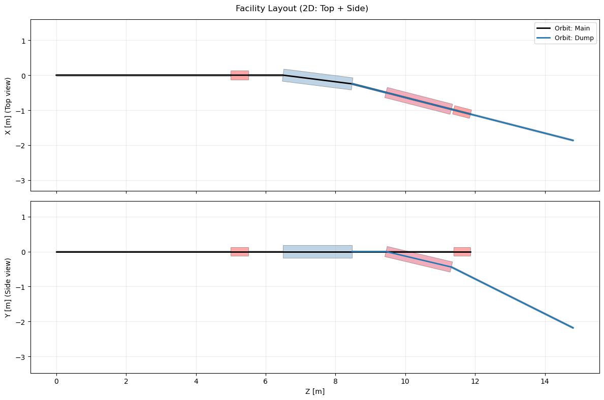
2D visualization

2D plotting typically provides:

• Top view: X vs Z
• Side view: Y vs Z

This representation is well suited for:

• quick geometry checks
• publications and reports
• debugging beamline curvature

Aspect ratios can be enforced so that transverse dimensions are not distorted.

fig, (ax_top, ax_side) = plot_layout_2d(
    facility,
    show_orbit=True,
    show_elements=True,
    equal_aspect=True,
    title="Facility Layout (2D: Top + Side)"
)

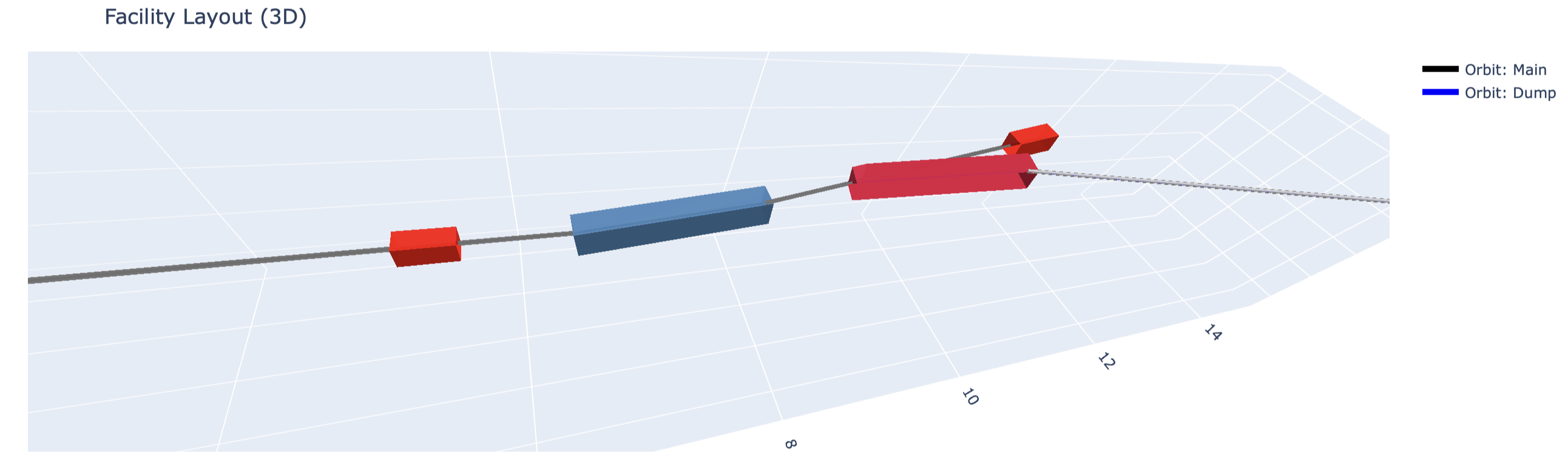
3D visualization (Plotly)

3D visualization provides an intuitive representation of the entire facility:

• reference trajectories are drawn as lines
• elements are rendered as boxes or cylinders
• visual dimensions are controlled via element attributes

Important implementation details:

• element bodies are positioned using r_start and W_start
• X and Y axes are scaled equally so that round elements remain round
• element geometry is rigidly attached to the beamline orientation

---

Visualization-only element attributes

Starting from Ocelot version ≥ 25.12, elements support additional attributes used only for visualization:

• width — transverse size in the x-direction
• height — transverse size in the y-direction
• color — display color for plotting

These attributes do not affect beam dynamics or tracking.

---

fig = plot_layout_3d(
    facility,
    show_orbit=True,
    show_elements=True,
    title="Facility Layout (3D)"
)
fig.show()

Interference checks

check_interferences() computes minimum distance between element centerline segments of different beamlines.

This is a coarse check (segment-to-segment distance + width-based radius), but very useful to catch obvious overlaps.

collisions = facility.check_interferences(min_distance=0.10)

if collisions:
    print(f" Found {len(collisions)} collisions:")
    for (lineA, elA, lineB, elB, dist) in collisions:
        print(f"  {lineA}.{elA} <-> {lineB}.{elB}  dist={dist:.4f} m")
else:
    print(" No collisions detected.")

      Found 3 collisions:
      Main.b1 <-> Dump.dd1  dist=0.0000 m
      Main.d3 <-> Dump.dd1  dist=0.0000 m
      Main.d3 <-> Dump.db1  dist=0.0000 m

Practical tips

1) Using tilt

• Quad: tilt = π/4 → skew quad (visual + optics meaning)
• Bend: tilt = π/2 → vertical bend (survey & visual)

2) Choosing width and height

• Use physical magnet yoke size if you want realistic pictures.
• If you just want readability, pick a few standard sizes:
  • drifts/cavities: ~0.1–0.2 m
  • quads/sexts: ~0.2–0.4 m
  • bends: ~0.3–0.6 m

3) Anchor semantics for branches

A child line starts at the exit of the anchor element in the parent line and inherits the parent’s orientation at that point.